27 Oct 2026

Kategorna logika (Simpson)

Lecture 1 - Algebraic theories

We are interested in a few perspectives.

Algebraic structure on sets vs on "spaces"
In what generality can we interpret algebraic structure?
When are two notions of algebra equivalent
Categorification: Presenting mathematical structures through the lens of category theory. For instance, we can look at an algebraic theory as a Lawvere theory. Here categories of algebras are looked at as functor categories (we call this functorial semantics).

We usually define a group as a structured set. This can be put in a categorical way thus.

A group is a set $G$ with

\begin{align*} m &: G \times G \rightarrow G & & m : G^2 \rightarrow G \\ e &\in G & & e : G^0 \rightarrow G \\ i &: G \rightarrow G & & i : G^{1} \rightarrow G \end{align*}

which satisfies

(associativity) $m(x, m(y, z)) = m(m(x, y), z)$
(unit) $m(e, x) = x = m(x, e)$
(inverse) $m(i(x), x) = e = m(x, i(x))$

Giving the definition like this, where we express all of the operations and structure as morphism, we can easily transfer the definition into other contexts, for instance, topological spaces, giving us topological groups.

This is instantiating the same concept in two categories, i.e. the category of sets and the category of topological spaces.

A group object in a category $\mathcal{C}$ with finite products is an object $G$ along with morphisms

\begin{align*} m &: G \times G \rightarrow G \\ e &: 1 \rightarrow G \\ i &: G \rightarrow G \end{align*}

satisfying associativity, given by the diagram

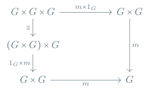$\begin{tikzcd} {G \times G \times G} && {G\times G} \\ {(G\times G)\times G} \\ {G\times G} && G \arrow["{m \times 1_G}", from=1-1, to=1-3] \arrow["\cong"', from=1-1, to=2-1] \arrow["m", from=1-3, to=3-3] \arrow["{1_G\times m}"', from=2-1, to=3-1] \arrow["m"', from=3-1, to=3-3] \end{tikzcd}$ and likewise satisfying diagrams for unit and inverse.

This defines a category of group objects.

The category $\Cat{Grp}_{\mathcal{C}}$ of group objects in $\mathcal{C}$ is given by the group objects $(G, m, e, i)$ as the objects, and the morphisms $(G, m, e, i) \rightarrow (G', m', e', i')$ being specified as $\mathcal{C}$-morphisms $G \xrightarrow{h} G'$ such that

$\begin{tikzcd} {G\times G} && {G'\times G'} &&& 1 &&& G && {G'} \\ \\ G && {G'} && G && {G'} && G && {G'} \arrow["{h\times h}", from=1-1, to=1-3] \arrow["m"', from=1-1, to=3-1] \arrow["{m'}", from=1-3, to=3-3] \arrow["e"', from=1-6, to=3-5] \arrow["{e'}", from=1-6, to=3-7] \arrow["h", from=1-9, to=1-11] \arrow["i"', from=1-9, to=3-9] \arrow["{i'}", from=1-11, to=3-11] \arrow["{h'}"', from=3-1, to=3-3] \arrow["h"', from=3-5, to=3-7] \arrow["h"', from=3-9, to=3-11] \end{tikzcd}$

Where identities and composition work as expected.

An algebraic signature $\Sigma$ is a colletion of operations where each operation $f$ has an associated arity $k \in \N$. Here constants are interpreted as having arity $k = 0$.

The terms $t$ are built by

variables $x$ are terms
if $t_1, \dots, t_k$ are tems and $f$ is an operation of arity $k$, then \[ f(t_1, \dots, t_k) \] is a term.

We will write $t \quad (x_1, \dots, x_n)$ to mean all variabels in $t$ are contained in the set $\left\{ x_1, \dots, x_n \right\}$.

An equation is then a pair of terms $t, t'$ written as $t = t' \quad (x_1, \dots, x_n)$. We might omit the context of the variables on the right on occasiond.

An algebraic theory $T$ is then given as $T = \Sigma + \mathcal{E}$, i.e. as a signature and set of equations $\mathcal{E}$.

A $T$-object in $\mathcal{C}$ with finite products is given by

an object $A$ of $\mathcal{C}$
for every operation $f \in \Sigma$ of arity $k$, a chosen morphism $f^A : A^k \rightarrow A$

such that all equations in $\mathcal{E}$ are true in $A$.

In particular, we interpret any term $t\quad (x_1, \dots, x_n)$ as a morphism $t^A : A^n \rightarrow A$. The interpretation is given as

\begin{align*} A^n \xrightarrow{x_i} A &\coloneqq A^n \xrightarrow{\pi_i} A \\ A^n \xrightarrow{f(t_1, \dots, t_k)^A} A & \coloneqq A^n \xrightarrow{t_1^A, \dots, t_k^A} A^k \xrightarrow{f^A} A \end{align*}

An equation $t = t' \quad (x_1, \dots, x_n)$ is satisfied if \[ A^n \xrightarrow{t^A} A = A^n \xrightarrow{(t')^A} A. \]

The category $\Cat{Mod}(T, \mathcal{C})$ of $T$-objects in $\mathcal{C}$ is given by taking as the objects the $T$-objects in $\mathcal{C}$, i.e. $(A, (f^A)_{f \in \Sigma})$ and as morphisms \[ (A, (f^A)_{f \in \Sigma}) \rightarrow (B, (f^B)_{f \in \Sigma}) \] the $\mathcal{C}$-morphisms $A \xrightarrow{h} B$ such that for any $f \in \Sigma$ of arity $k$, we have that

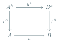$\begin{tikzcd} {A^k} && {B^k} \\ \\ A && B \arrow["{h^k}", from=1-1, to=1-3] \arrow["{f^A}"', from=1-1, to=3-1] \arrow["{f^B}", from=1-3, to=3-3] \arrow["h"', from=3-1, to=3-3] \end{tikzcd}$ commutes. Again the identities and compositions are as expected.

We define the Lawvere theory $\mathbb{T}$ of an algebraic theory $T = (\Sigma, \mathcal{E})$ as having

the objects $\underline{n}$ for $n \in \N$
and the morphisms being maps $\underline{m} \rightarrow \underline{n}$ given as $n$-tuples $([t_1], \dots, [t_n])$ where $t_1, \dots, t_n \quad (x_1, \dots, x_n)$.

Here $[t_i]$ mean the equivalence classes of terms modulo provable equality from $\mathcal{E}$.
The identities are given as \[ \underline{n} \rightarrow \underline{n} \coloneqq \underline{n} \xrightarrow{([x_1], \dots, [x_n])} \underline{n} \]
Composition of \[ \underline{n} \xrightarrow{([t_1], \dots, [t_m]) \quad (x_1, \dots, x_l)} \underline{m} \xrightarrow{([t'_1], \dots, [t'_n]) \quad (x_1, \dots, x_m)} \underline{n} \] is given as \[ \underline{l} \xrightarrow{([t_1'[t_1, \dots, t_m / x_1,\dots, x_m]], \dots)} \underline{n} \] i.e. a substitution.

Algebraic theories $T$ and $T'$ are equivalent if $\mathbb{T} \simeq \mathbb{T}'$ are equivalent categories.

Note that $\mathbb{T}$ has finite products, the terminal object is $1 = \underline{0}$ and $\underline{m} \times \underline{n} = \underline{m + n}$.

The Lawvere theory of an algebraic theory is an instance of a syntactic category

\[ \Cat{Mod}(T, \mathcal{C}) \simeq \mathrm{FP}[\mathbb{T}, \mathcal{C}] \] where $\mathrm{FP}(\mathbb{T}, \mathcal{C})$ is the category given as finite-product-preserving functors $\mathbb{T} \rightarrow \mathcal{C}$ and the morphisms are natural transformations.

That a functor $F: \mathcal{C} \rightarrow \mathcal{D}$ over categories with finite products preserves finite products means that

\begin{align*} F(1_{\mathcal{C}}) &\cong 1_{\mathcal{D}} \\ F(X \times_{\mathcal{C}} Y) &\cong F(X) \times_{\mathcal{D}} F(Y) \end{align*}

Lecture 2 - Simply typed lambda calculus in CCCs

See also Lecture 5: Lambda račun s preprostimi tipi from TPJ (in Slovene) for a more "direct" treatment.

An exponential $Y^X$ for objects $X, Y$ of a category $\mathcal{C}$ is an evaluation map \[ Y^X \times X \xrightarrow{\epsilon_{X, Y}} Y \] such that for any \[ Z^X \times X \xrightarrow{f} Yn \] there exists a unique $Z \xrightarrow{\Lambda_f} Y^X$ satisfying

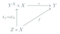
$\begin{tikzcd} {Y^X \times X} && Y \\ \\ {Z \times X} \arrow["\epsilon", from=1-1, to=1-3] \arrow["{\Lambda_f\times \operatorname{id}_X}", from=3-1, to=1-1] \arrow["f"', from=3-1, to=1-3] \end{tikzcd}$

Importantly, exponentials are unique up to isomorphism. Specifically, suppose $X \Rightarrow Y \times x \xrightarrow{\epsilon} Y$ and $X \Rightarrow' Y \times X \xrightarrow{\epsilon'} Y$ are both exponentials. Then \[ (X \Rightarrow' Y) \xrightarrow{\Lambda \epsilon'} (X \Rightarrow Y) \] and \[ (X \Rightarrow' Y) \xleftarrow{\Lambda \epsilon} (X \Rightarrow Y) \] is a pair of an isomorphisms.

A cartesian-closed category is a category with finite products and all exponentials.

$\Cat{Set}$ is the prototypical example of a ccc.
Categories of presheaves and sheaves (which we will come to)
Boolean algebras and more generally Heyting algebras.
$\Cat{Cat}$, the category of categories

An important nonexample we will come to are topological spaces with the compact open topology.

An object $X$ is exponentiable if for any $Y \in \abs{\mathcal{C}}$, the exponential $Y^X$ exists.

If $X$ is exponentiable, then we can view the mapping $(-)^X : \Cat{C} \rightarrow \Cat{C}$ as an endofunctor. The object action maps $Y$ to $Y^X$, and the morphism action maps $f : Y \rightarrow Y'$ to \[ \Lambda(f \circ \epsilon_{X, Y}) : Y^X \rightarrow (Y')^X \] This gives the characterisation that $X$ is exponentiable if and only if the functor $(-) \times X$ has a right adjoint, in which case $(-) \times X \dashv (-)^X$.

In $\Cat{Top}$ a space $X$ is exponentiable if and only if it is core compact (a generalization of local compactness). Not every space is core compact, hence $\Cat{Top}$ is not cartesian closed.

Because of this, we consider so called convenient categories of topological spaces.

A collection $\operatorname{Base}$ of base types. Then we can form more types as \[ A, B, \dots \Coloneqq a \in \operatorname{Base} \mid A \times B \mid \underline{1} \mid A \rightarrow B \]

We also have a collection of terms. There is a judgement $\Gamma \vdash t : A$ which says that $t$ is an element of type $A$ in context $\Gamma$. A context $\Gamma$ is a collection $x_1 : A_1, \cdots, x_k : A_k$ for $k \geq 0$ such that $i \neq j \implies x_i \neq x_j$.

Terms are specified by axioms, introduction rules, and elimination rules. First, for every $1 \leq i \leq k $ we have \[

\begin{bprooftree} \AxiomC{} \UnaryInfC{$x_1 : A_1, \cdots, x_k : A_k \vdash x_i : A_i$ } \end{bprooftree}

\] Products are specified by the introduction rule \[

\begin{bprooftree} \AxiomC{$\Gamma \vdash s : A$} \AxiomC{$\Gamma \vdash t : B$} \RightLabel{$\times$-intro} \BinaryInfC{$\Gamma \vdash (s, t) : A \times B$} \end{bprooftree}

\] and the elimination rules \[

\begin{bprooftree} \AxiomC{$\Gamma \vdash t : A_1 \times A_2$} \RightLabel{$\times$-elim} \UnaryInfC{$\Gamma \vdash \pi_i t : A_i$ } \end{bprooftree}

The terminal type is given by \[

\begin{bprooftree} \AxiomC{} \RightLabel{$\underline{1}$-intro} \UnaryInfC{$\Gamma \vdash \star : \underline{1}$ } \end{bprooftree}

Most importantly, lambda terms introduce as \[

\begin{bprooftree} \AxiomC{$\Gamma, x : A \vdash t : B$} \RightLabel{$\rightarrow$-intro} \UnaryInfC{$\Gamma \vdash \lambda x : A .\, t : A \rightarrow B$ } \end{bprooftree}

\] and eliminate as \[

\begin{bprooftree} \AxiomC{$\Gamma \vdash s : A \rightarrow B$} \AxiomC{$\Gamma \vdash t : A$} \RightLabel{$\rightarrow$-elim} \BinaryInfC{$\Gamma \vdash st : B$} \end{bprooftree}

There are also equality rules we must consider (they are in the notes). But in particular we have equality judgements \[ \Gamma \rightarrow s = t : A \] presupposing $\Gamma \vdash s : A$ and $\Gamma \vdash t : A$. This gives rise to 4 kinds of equality judgements. Firstly, that equality is an equivalence relation \[

\begin{bprooftree} \AxiomC{$\Gamma \vdash t : A$} \UnaryInfC{$\Gamma \vdash t = t : A$ } \end{bprooftree}

\quad

\begin{bprooftree} \AxiomC{$\Gamma \vdash s = t : A$} \UnaryInfC{$\Gamma \vdash t = s : A$ } \end{bprooftree}

\quad \text{transitivity} \]

And also of a congruence relation, i.e. \[

\begin{bprooftree} \AxiomC{$\Gamma \vdash s = s' : A$} \AxiomC{$\Gamma \vdash t = t' : B$} \BinaryInfC{$\Gamma \vdash (s, t) = (s', t') : A \times B$} \end{bprooftree}

\] and \[

\begin{bprooftree} \AxiomC{$\Gamma, x : A \vdash t = t' : B$} \UnaryInfC{$\Gamma \vdash \lambda x : A .\, t = \lambda x : A.\, t' : A \rightarrow B$ } \end{bprooftree}

Note that the name of the variable in the definition didn't really matter. This notion gives rise to the $\beta$-rules \[

\begin{bprooftree} \AxiomC{$\Gamma \vdash t_1 : A_1$} \AxiomC{$\Gamma \vdash t_2 : A_2$} \RightLabel{$i \in \left\{ 1, 2 \right\}$} \BinaryInfC{$\Gamma \vdash \pi_i(t, t_2) = t_i : A_i$} \end{bprooftree}

\] and \[

\begin{bprooftree} \AxiomC{$\Gamma, x : A \vdash s : B$} \AxiomC{$\Gamma \vdash t : A$} \BinaryInfC{$\Gamma \vdash (\lambda x : A.\, s) t = s[t/x] : B$} \end{bprooftree}

\] where $s[t/x]$ means $t$ substituted for the variable $x$. We may assume bound variables in $s$ are renamed before the substitution.

We also have $\eta$ rules. \[

\begin{bprooftree} \AxiomC{$\Gamma \vdash u : \underline{1}$} \UnaryInfC{$\Gamma \vdash u = \star : 1$ } \end{bprooftree}

\quad

\begin{bprooftree} \AxiomC{$\Gamma \vdash u : A \times B$} \UnaryInfC{$\Gamma \vdash u = (\pi_1 u, \pi_2 u) : A \times B $} \end{bprooftree}

\] and \[

\begin{bprooftree} \AxiomC{$\Gamma \vdash u : A \rightarrow B$} \RightLabel{$x \not\in \Gamma$} \UnaryInfC{$\Gamma \vdash u = \lambda x : A.\, (ux) : A \rightarrow B$ } \end{bprooftree}

The fact that $\Gamma \vdash s[t/x] : B$ holds needs to be proved. This is the substitution lemma proved by induction on the structure of $s$.

We specify the theory of the simply typed $\lambda$-calculus as $T = (\operatorname{Base}, \Sigma, \mathcal{E})$. Here

$\operatorname{Base}$ is a set (of base types)
$\Sigma$ is a signature with elements $c : A$ such that each each $c$ in $\Sigma$ has only one type $A$. We add a rule \[
\begin{bprooftree} \AxiomC{} \RightLabel{$c : A \in \Sigma$} \UnaryInfC{$\Gamma \vdash c : A$ } \end{bprooftree}
\]
$\mathcal{E}$ is a set of typed equations $\Gamma \vdash s = t : A$ between terms $\Gamma \vdash s, t : A$. We add a rule \[
\begin{bprooftree} \AxiomC{} \RightLabel{$\Gamma \vdash s = t : A \in \mathcal{E}$} \UnaryInfC{$\Gamma \vdash s = t : A$ } \end{bprooftree}
\]

$\lambda$-theory of an algebraic theory

Every algebraic theory $(\Sigma_a, \mathcal{E}_a)$ gives us a $\lambda$-theory. We take $\operatorname{Base} = \left\{ a \right\}$. For every operation $f$ of arity $k$ we have $c_f : \underbrace{a \times \cdots \times a}_{k} \rightarrow a$. For every equation $t = t'$ with variables $x_1, \dots, x_k$ we add the equation \[ x_1 : a, \dots, x_k : a \vdash t = t' : a. \]

Gödel's system T

We take $\operatorname{Base} = \left\{ \underline{N} \right\}$, thinking of $\underline{N}$ as natural numbers.
The signature is $0 : \underline{N}, \operatorname{succ} : \underline{N} \rightarrow \underline{N}$, and a family of recursors \[ \left\{ R_A : A \rightarrow (A \rightarrow A) \rightarrow (\underline{N} \rightarrow A) \right\} \]
and equations
\begin{align*} \mathcal{E} = & x : A, f : A \rightarrow A \vdash R_A\, x \, f\, 0 = x : A\\ & x : A, f : A \rightarrow A, n : \underline{N} \vdash R_A \, x \, f \, (\operatorname{succ} n) = f(R_a \, x \, f\, n) : A \end{align*}

A $T$-model for $T = (\operatorname{Base}, \Sigma, \mathcal{E})$ in a CCC $\mathcal{C}$ is given by:

An interpretaton $a^{\mathcal{C}} \in \abs{\mathcal{C}}$ for every $a \in \operatorname{Base}$ Note that this determines an interpretation of $A^{\mathcal{C}}$ of any type $A$.
\begin{align*} (A \times B)^{\mathcal{C}} &\coloneqq A^{\mathcal{C}} \times B^{\mathcal{C}} \\ \underline{1}^{\mathcal{C}} &\coloneqq \underline{1} \\ (A \rightarrow B)^{\mathcal{C}} &\coloneqq (B^{\mathcal{C}})^{(A^{\mathcal{C}})} \end{align*}
For a typed constant $C : A \in \Sigma$, we define $\underline{1} \xrightarrow{C^A} A^{\mathcal{C}}$. This way constants are interpreted as global elements. This also leads to determining the rest of the terms.
Contexts are interpreted inductively by
\begin{align*} ()^{\mathcal{C}} &\coloneqq \underline{1} \\ \Gamma, x : A &\coloneqq \Gamma^{\mathcal{C}} \times A^{\mathcal{C}} \end{align*}
Essentially contexts are iterated products.
In general, a term $\Gamma \vdash t : A$ will be interpreted as a morphism \[ \Gamma^{\mathcal{C}} \xrightarrow{(\Gamma \vdash t : A)^{\mathcal{C}}} A^{\mathcal{C}} \] This involves a lenghty definition, so we will leave it out for now.
The construction is subject to the condition that for every equation $\Gamma \vdash_T s = t : A \in \mathcal{E}$ provable in $T$, it holds that \[ (\Gamma \vdash s : A)^{\mathcal{C}} = (\Gamma \vdash t : A)^{\mathcal{C}}. \] This means that our interpretation works in a way which makes the equations of our theory true.

Soundness & completeness

The following are equivalent

$\Gamma \vdash_T s = t : A$, i.e. equations provable in $T$, i.e. from $\mathcal{E}$
For evrey CCC $\mathcal{C}$ and every $T$-model in $\mathcal{C}$ \[ (\Gamma \vdash s : A)^{\mathcal{C}} = (\Gamma \vdash t : A)^{\mathcal{C}} : \Gamma^{\mathcal{C}} \rightarrow A^{\mathcal{C}} \]

We call $(1) \implies (2)$ soundness and $(2) \implies (1)$ completeness.

Lecture 3 - Monads and their algebras

In any category $\mathcal{C}$ with fine products and algebraic theory $T = (\Sigma, \mathcal{E})$, a $T$-algebra is a pair $(A, (m^A)_{m \in \Sigma})$. We name the category $\Cat{Alg}_T(\mathcal{C})$ of $T$-algebras in $\mathcal{C}$ and their homomorphisms.

Given an object $X \in \abs{\mathcal{C}}$, the free $T$-algebra in $\mathcal{C}$ over $X$, if it exists, is given by a $T$-algebra $(FX, (f^{FX})_{f \in \Sigma})$ and a map $X \xrightarrow{\eta_X} FX$ called the insertion of generators, such that for any other pair $(A, (f^A)_f)$ and map $X \xrightarrow{g} A$, there exists a unique homomorphism $h : (FX, (f^{FX})_f) \rightarrow (A, (f^A)_{f})$ such that

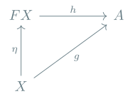$\begin{tikzcd} FX && A \\ \\ X \arrow["h", from=1-1, to=1-3] \arrow["\eta", from=3-1, to=1-1] \arrow["g"', from=3-1, to=1-3] \end{tikzcd}$ commutes.

This definition determines the free algebra up to isomorphism. We also say $\mathcal{C}$ has free $(\Sigma, \mathcal{E})$-algebras if it has free algebras over every object $X$.

Free groups

Remember the free group is constructed as the set of irreducible words over $X \uplus X^{-1}$ with insertion of generators.

More generally, free $(\Sigma, \mathcal{E})$-algebras in $\Cat{Set}$ are constructed by \[ FX = \frac {\text{the set of terms with no variables over } \Sigma \uplus \left\{ c_x \mid x \in X \right\}}{\text{derivable equality from the equations in $\mathcal{E}$}} \] where $c_x$ are new constants, one for each $x \in X$.

Here we have \[ f^{FX}([t_1], \dots, [t_k]) = [f(t_1, \dots, t_k)]. \] and \[ \eta^X(x) = [c_x]. \]

$\Cat{Set}$ then has free $(\Sigma, \mathcal{E})$-algebras.

Suppose $\mathcal{C}$ has free $T$-algebras. Further supose we have a choice of $(FX, (f^{FX}))$ for every object $X \in \abs{\mathcal{C}}$. Then $F$ defines a functor $\mathcal{C} \rightarrow \Cat{Alg}_T(\mathcal{C})$, that is, the free-algebra functor.

By the universal property of algebras, there exists a unique $h$ such that

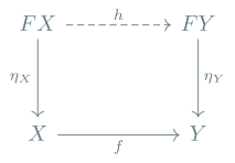$\begin{tikzcd} FX && FY \\ \\ X && Y \arrow["h", dashed, from=1-1, to=1-3] \arrow["{\eta_X}"', from=1-1, to=3-1] \arrow["{\eta_Y}", from=1-3, to=3-3] \arrow["f"', from=3-1, to=3-3] \end{tikzcd}$ commutes, which allows us to define the morphism action as

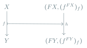
$\begin{tikzcd} X && {(FX, (f^{FX})_f)} \\ \\ Y && {(FY, (f^{FY})_f)} \arrow[""{name=0, anchor=center, inner sep=0}, "f"', from=1-1, to=3-1] \arrow[""{name=1, anchor=center, inner sep=0}, "h", from=1-3, to=3-3] \arrow[between={0.2}{0.8}, maps to, from=0, to=1] \end{tikzcd}$

We also have an obvious functor $U : \mathcal{Alg}_T(\mathcal{C}) \rightarrow \mathcal{C}$ called the forgetful functor.

By this construction, we see that $\eta : \mathrm{Id}_{\mathcal{C}} \rightarrow UF$.

Remember the definition of adjunction.

$F : \mathcal{C} \rightarrow \mathcal{D}$ is left adjoint to $G : \mathcal{D} \rightarrow \mathcal{C}$, $F \dashv G : \mathcal{D} \rightarrow \mathcal{C}$ if there exist bijections \[ \Psi_{X, Y} : \mathcal{D}(FX, Y) \xrightarrow{\cong} \mathcal{C}(X, GY) \] natural in $X$ and $Y$.

There is an equivalent characterization in terms of the existence of some specific transformations.

We have that $F \dashv G$ if and only if there exist natural transformations $\eta : \operatorname{id}_{\mathcal{C}} \Rightarrow GF$ called the unit and $\varepsilon :FG \Rightarrow \operatorname{id}_{\mathcal{D}}$ called the counit of the adjunction, such that

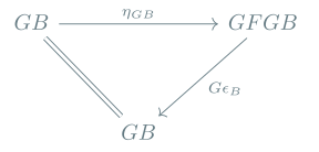
$\begin{tikzcd} GB && GFGB \\ \\ & GB \arrow["\eta_{GB}", from=1-1, to=1-3] \arrow["{G\epsilon_B}", from=1-3, to=3-2] \arrow[equal, from=1-1, to=3-2] \end{tikzcd}$

and

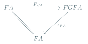
$\begin{tikzcd} FA && FGFA \\ \\ & FA \arrow["{F\eta_A}", from=1-1, to=1-3] \arrow["{\epsilon_{FA}}", from=1-3, to=3-2] \arrow[equal, from=1-1, to=3-2] \end{tikzcd}$

commute for all $A \in \abs{\mathcal{C}}$and $B \in \abs{\mathcal{D}}$.

We have $F \dashv U : \Cat{Alg}_T(\mathcal{C}) \rightarrow \mathcal{C}$.

Define

\begin{align*} \Psi : \Cat{Alg}_T(\mathcal{C})((FX, (f^{FX})_f), (A, (f^A)_f)) &\rightarrow \mathcal{C}(X, A) \\ (FX, -) \xrightarrow{h} (A, -) &\mapsto h \circ \eta_X \\ \text{ unique $h$ from the u.p.} &\mapsfrom g \end{align*}

Here the unit is $X \xrightarrow{\eta_X} UFX$.

In the case of $(\Sigma, \mathcal{E})$ on $\mathcal{Set}$, we have a so-called monadic structure.

$FX$ is equivalence classes $[t]$ on terms $t$ over $\Sigma \uplus \left\{ c_x \mid x \in X \right\}$
$FFX$ are equivalence classes $[t]$ of terms $t$ over $\Sigma \uplus \left\{ c_{[t]} \mid [t] \in FX \right\}$

Then for $\mu_X : FFX \rightarrow FX$ we have

\begin{align*} \mu_X[c_{[t]}] &= [t] \\ \mu_X[f([t_1], \dots, [t_k])] &= [f(t_i', \dots, t_k')] \end{align*}

where $t_i'$ is such that $\mu_x[t_i] = [t_i']$

A monad on a category $\mathcal{C}$ is a functor $T : \mathcal{C} \to \mathcal{C}$ together with:

A natural transformation $\eta : 1 \Rightarrow T$ called the unit of the monad
A natural transformation $\mu : T^2 \Rightarrow T$ called the multiplication of the monad.

We say the monad is the triple $(T, \eta, \mu)$.

satisfying the following commutative diagrams for all objects $X$ of $\mathcal{C}$:

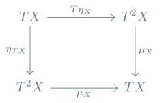
$\begin{tikzcd} TX && {T^2X} \\ \\ {T^2X} && TX \arrow["{T\eta_X}", from=1-1, to=1-3] \arrow["{\eta_{TX}}"', from=1-1, to=3-1] \arrow["{\mu_X}", from=1-3, to=3-3] \arrow["{\mu_X}"', from=3-1, to=3-3] \end{tikzcd}$

and

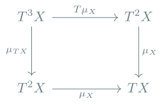
$\begin{tikzcd} T^3X && T^2X \\ \\ T^2X && TX \arrow["T\mu_X", from=1-1, to=1-3] \arrow["{\mu_{TX}}"', from=1-1, to=3-1] \arrow["\mu_X", from=1-3, to=3-3] \arrow["\mu_X"', from=3-1, to=3-3] \end{tikzcd}$

An Eilenberg-Moore algebra for a monad $T$ is $A, a$ where $A \in \mathcal{C}$ and $a : TA \rightarrow A$ in $\mathcal{C}$ is a map such that

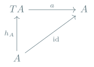$\begin{tikzcd} TA && A \\ \\ A \arrow["a", from=1-1, to=1-3] \arrow["{h_A}", from=3-1, to=1-1] \arrow["{\operatorname{id}}"', from=3-1, to=1-3] \end{tikzcd}$ and

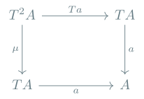$\begin{tikzcd} {T^2A} && TA \\ \\ TA && A \arrow["Ta", from=1-1, to=1-3] \arrow["\mu"', from=1-1, to=3-1] \arrow["a", from=1-3, to=3-3] \arrow["a"', from=3-1, to=3-3] \end{tikzcd}$ commute.

An algebra homomorphism $h : (A, a) \rightarrow (B, b)$ is a map $h$ in $\mathcal{C}$ such that

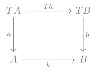$\begin{tikzcd} TA && TB \\ \\ A && B \arrow["Th", from=1-1, to=1-3] \arrow["a"', from=1-1, to=3-1] \arrow["b", from=1-3, to=3-3] \arrow["h"', from=3-1, to=3-3] \end{tikzcd}$ commutes.

This means EM algebras form a category, which we call the Eilenberg-Moore category and denote it $\mathcal{C}^T$.

We define a comparison functor $K : \Cat{Alg}_{(\Sigma, \mathcal{E})}(\mathcal{C}) \rightarrow \mathcal{C}^T$. NB these exist for any codomain of the right adjoint.

Then $(A, (f^A)_f) \mapsto (A, TA \xrightarrow{a_A} A)$, where $TA \xrightarrow{a_A} A$ is the unique homomorphism $(FA, (f^{FA})_f) \rightarrow (A, (f^A)_f)$ such that

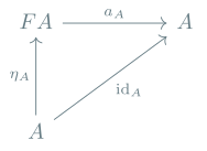
$\begin{tikzcd} FA && A \\ \\ A \arrow["{a_A}", from=1-1, to=1-3] \arrow["{\eta_A}", from=3-1, to=1-1] \arrow["{\operatorname{id}_A}"', from=3-1, to=1-3] \end{tikzcd}$

This is indeed an EM-algebra, the operation extends to a functor. This holds in general for any adjunction $F \dashv U$.

Specific to $\Cat{Algebra_{(\Sigma, \mathcal{E})}}(\mathcal{C})$ is also the fact that this functor is full and faithful.

For $\mathcal{C} = \mathcal{Set}$, $K : \Cat{Algebra_{(\Sigma, \mathcal{E})}}(\Cat{Setsn}) \rightarrow \Cat{Set}^T$ is an isomorphism of categories.

We can prove this using Beck's theorem (characterizing monadicity). The theorem is one part of Linton's theorems.

Lecture 4 - Computational effects and monads

We think of pure computation as computing functions in the mathematical sense as morphisms $A \rightarrow B$. Today we will consider computational effects which extend this theory.

A very simple notion of an effect is partiality $A \rightharpoonup B$. Note it is equivalent to consider maps $A \rightarrow B_{\bot} = B \uplus \left\{ \bot \right\}$.
Probabilistic computation can likewise be considered as an effect as mapping into (discrete) probability distributions $A \rightarrow D(B)$, where $D(B) = \left\{ d : B \rightarrow [0, 1] \mid \sum\limits_{b \in B}^{} d(b) = 1 \right\}$. These two may be combined.
Nondeterminism is modeled as $A \rightarrow \pot^{ + }(B)$.
A particularly relevant exaple is output $A \rightarrow \Sigma^{ * } \times B$.
Computers have internal state. We can model stateful computation as \[ S \times A \rightarrow S \times B. \] Note this is equivalent to considering maps \[ A \rightarrow (S \times B)^S. \]
Continuations $(B \rightarrow R) \rightarrow (A \rightarrow R)$, which we can view as a function \[ A \rightarrow R^{R^B}. \] Interestingly, this also has algebraic implications.

All of these examples have the form $A \rightarrow TB$ where $T$ is a monad. Computations are then Kleisli maps.

We consider the language with types \[ A \Coloneqq a \in \operatorname{Base} \mid A \times B \mid A \rightarrow B \mid \underline{1} \mid TA \] and typed terms $\Gamma \vdash t : A$ over a context, as well as the following rules.

\begin{gather*} \begin{bprooftree} \AxiomC{$\Gamma \vdash t : A$} \UnaryInfC{$\Gamma \vdash \operatorname{return} t : TA$ } \end{bprooftree} \quad \begin{bprooftree} \AxiomC{$\Gamma \vdash s : TA$} \AxiomC{$\Gamma, x : A \vdash t : TB$} \BinaryInfC{$\Gamma \vdash \operatorname{do} x \leftarrow s \operatorname{in} t : TB$} \end{bprooftree} \end{gather*}

There are some meta-theoretic properties we can prove for any such system.

(Weakening) If $\Gamma \vdash t : A$ for $\Gamma \subseteq \Gamma'$, we can derive \[ \Gamma' \vdash t : A \]
(Uniqueness of typing) If $\Gamma \vdash t : A$ and $\Gamma \vdash t : A'$, then $A \equiv A'$.
Substitution, from last week.

We also have equalities $\Gamma \vdash s = t : A$ where we require $\Gamma \vdash s : A$ and $\Gamma \vdash t : A$. Congruence and the equivalence relation properties are as before. We add things like \[

\begin{bprooftree} \AxiomC{$\Gamma \vdash s = s' : TA$} \AxiomC{$\Gamma, x : A \vdash t = t' : TB$} \BinaryInfC{$\Gamma \vdash (\operatorname{do} x \leftarrow s \operatorname{in} t) = (\operatorname{do} x \leftarrow s' \operatorname{in} t') : TB$ } \end{bprooftree}

We also have the $\beta$-rules \[

\begin{bprooftree} \AxiomC{$\Gamma \vdash s : A$} \AxiomC{$\Gamma, x : A \vdash t : TB$} \BinaryInfC{$\Gamma \vdash \operatorname{do} x \leftarrow \operatorname{return} s \operatorname{in} t = t[s/x] : TB$} \end{bprooftree}

\] and the $\eta$-rule \[

\begin{bprooftree} \AxiomC{$\Gamma \vdash u : TA$} \UnaryInfC{$\Gamma \vdash u = \operatorname{do} x \leftarrow u \operatorname{in} \operatorname{return} x : TA$ } \end{bprooftree}

Unlike with the STLC, in this case, we require one more rule, namely associativity of Kleisli composition. \[

\begin{bprooftree} \AxiomC{$\Gamma \vdash s : TA$} \AxiomC{$\Gamma, x : A \vdash t : TB$} \AxiomC{$\Gamma, y : B \vdash u : TC$} \TrinaryInfC{$\overset{\Gamma \vdash \operatorname{do} x \leftarrow s \operatorname{in} (\operatorname{do} y \leftarrow t \operatorname{in} u)} {= \operatorname{do} y \leftarrow (\operatorname{do} x \leftarrow s \operatorname{in} t) \operatorname{in} : TC}$} \end{bprooftree}

A strong monad on $\mathcal{C}$ with finite products is $(T, \eta, \mu, t)$ where $T : C\rightarrow C$, $\eta_X : X \rightarrow TX$, $\mu_X : T^2X \rightarrow TX$ is a monad and $t_{X, Y} : X \times TY \rightarrow T(X \times Y)$ is a strength of the monad $T$, i.e. natural in $X$ and $Y$, and is a strength for the functor, namely

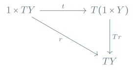$\begin{tikzcd} {1 \times TY} && {T(1 \times Y)} \\ \\ && TY \arrow["t", from=1-1, to=1-3] \arrow["r"', from=1-1, to=3-3] \arrow["Tr", from=1-3, to=3-3] \end{tikzcd}$ and

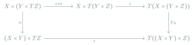$\begin{tikzcd} {X\times(Y\times TZ)} && {X \times T(Y\times Z)} && {T(X\times (Y \times Z))} \\ \\ {(X\times Y)\times TZ} &&&& {T((X \times Y) \times Z)} \arrow["{x\times t}", from=1-1, to=1-3] \arrow["a"', from=1-1, to=3-1] \arrow["t", from=1-3, to=1-5] \arrow["Ta", from=1-5, to=3-5] \arrow["t"', from=3-1, to=3-5] \end{tikzcd}$ It further respects the monad structure with

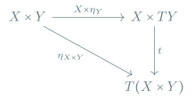$\begin{tikzcd} {X\times Y} && {X\times TY} \\ \\ && {T(X\times Y)} \arrow["{X\times\eta_Y}", from=1-1, to=1-3] \arrow["{\eta_{X\times Y}}"', from=1-1, to=3-3] \arrow["t", from=1-3, to=3-3] \end{tikzcd}$ and

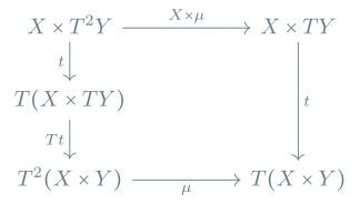
$\begin{tikzcd} {X\times T^2Y} && {X\times TY} \\ {T(X\times TY)} \\ {T^2(X\times Y)} && {T(X\times Y)} \arrow["{X\times \mu}", from=1-1, to=1-3] \arrow["t"', from=1-1, to=2-1] \arrow["t", from=1-3, to=3-3] \arrow["Tt"', from=2-1, to=3-1] \arrow["\mu"', from=3-1, to=3-3] \end{tikzcd}$

p NB a strength can also be defined for an arbitrary functor. It being a strength of a monad adds further coherence condition with the monad structure.

If a monoidal category is closed, strengths are in 1-to-1 correspondence with enrichments of the functor.

Strong monads allow us to give an interpretation of an algebra with the strong monad.

Suppose $\mathcal{C}$ is a CCC with a strong monad $(T, \eta, \mu, t)$. An interpretation of $(\operatorname{Base}, \Sigma, \mathcal{E})$ in $\mathcal{C}$ with $(T, \eta, \mu, t)$ is given as

Every base type $a \in \operatorname{Base}$ gives $a^{\mathcal{C}} \in \abs{\mathcal{C}}$. Define $A^{\mathcal{C}}$ using $(TA)^{\mathcal{C}} = T(A^{\mathcal{C}})$.
Every constant $c : A \in \Sigma$ is interpreted $c^{\mathcal{C}} \in \mathcal{C}(1, A^{\mathcal{C}})$.
This induces an interpretation on terms \[ (\Gamma \vdash t : A)^{\mathcal{C}} \in \mathcal{C}(\Gamma^{\mathcal{C}}, A^{\mathcal{C}}) \] defined as before, plus \[ (\Gamma \vdash \operatorname{return} s : TA)^{\mathcal{C}} = \Gamma^{\mathcal{C}} \xrightarrow{s^{\mathcal{C}}} A^{\mathcal{C}} \xrightarrow{\eta} TA^{\mathcal{C}} \]

We also define

\begin{align*} &(\Gamma \vdash \operatorname{do} x \leftarrow s \operatorname{in} u : TB)^{\mathcal{C}} = \\ &= \Gamma^{\mathcal{C}} \xrightarrow{(\operatorname{id}_{\Gamma^{\mathcal{C}}}, (\Gamma \vdash s : TA)^{\mathcal{C}}) } \Gamma^{\mathcal{C}} \times TA^{\mathcal{C}} \xrightarrow{t} T(\Gamma^{\mathcal{C}} \times A^{\mathcal{C}}) \xrightarrow{T(\Gamma, x : A \vdash u : TB)^{\mathcal{C}}} T^2 B^{\mathcal{C}} \xrightarrow{\mu} TB^{\mathcal{C}} \end{align*}

Soundness and completeness

The following are equivalent.

$\Gamma \vdash_{(\operatorname{Base}, \Sigma, \mathcal{E}) S_1 = S_2 : A}$
For all CCCs $\mathcal{C}$ and strong monads $T$ on $\mathcal{C}$, if al equations in $\mathcal{E}$ are true, then \[ \Gamma^{\mathcal{C}} \xrightarrow{S_1^{\mathcal{C}}} A^{\mathcal{C}} = \Gamma^{\mathcal{C}} \xrightarrow{S_2^{\mathcal{C}}} A^{\mathcal{C}} \]

The syntactic category for $\lambda_T$ has

types as objects
Morphisms $A \rightarrow B$ given as $[x : A \vdash t : B]$ which is an equivalence class modulo provable equality.
identity is given as $[x : A \vdash x : A] : A \rightarrow A$
Composition is given as \[ [y : B \vdash u : C] \circ [x : A \vdash s : B] \coloneqq [x : A \vdash u[s/y] : C]. \]

This is a CCC.

We have a strong monad on this syntactic category given by $T$ with morphism action

\begin{align*} (A \rightarrow B) &\longrightarrow (TA \rightarrow TB) \\ [x : A \vdash u : B] &\mapsto [y : TA \vdash \operatorname{do} x \leftarrow y \operatorname{in} \operatorname{return} u : TB] \end{align*}

The unit is given as \[ \eta_A : A \xrightarrow{[x : A \vdash \operatorname{return} x : TA]} TA \] The multiplication as \[ \mu_A : T^2A \xrightarrow{[x : T^2 A \vdash \operatorname{do} y \leftarrow x \operatorname{in} y]} TA \] And the strength is given as \[ t_{A, B} : A \times TB \xrightarrow{x : A \times TB \vdash \operatorname{do} y \leftarrow \pi_2 x \operatorname{in} \operatorname{return} (\pi_1 x, y) : T(A \times B)} T(A\times B) \]

Suppose $C$ is a category with a monad $(T, \eta, \mu)$. The Kleisli category $\mathcal{C}_T$ is given by

The objects of $\mathcal{C}_T$ are the objects of $\mathcal{C}$
The maps are $\mathcal{C}_T(A, B) = \mathcal{C}(A, TB)$.
The composition is given by kleisli composition. For $f : A \rightarrow TB$ and $g : B \rightarrow TC$, we have \[ g \circ_T f = A \xrightarrow{f} TB \xrightarrow{Tg} T^2C \xrightarrow{\mu} TC. \] We can verify associativity.
Identity is given simply as $A \xrightarrow{\eta_A} TA$.

We can think about also defining $\Gamma$-parametrised composition i.e. \[

\begin{bprooftree} \AxiomC{$\Gamma \times A \rightarrow TB$} \AxiomC{$\Gamma \times B \rightarrow TC$} \BinaryInfC{$\Gamma \times A \rightarrow TC$} \end{bprooftree}

Given any adjunction $F \dashv G : \mathcal{D} \rightarrow \mathcal{C}$, then $T = GF : \mathcal{C} \rightarrow \mathcal{C}$ gives a monad

$\eta_X : X \rightarrow TX$ is the unit of the adjunction
$\mu_X : T^2 \rightarrow TX := G\varepsilon_F$ withere $\varepsilon$ is the counit of the adjunction.

Then we get the following diagram, where we get $J$ and $K$ from the adjunctions.

$\begin{tikzcd} {\mathcal{C}_T} && {\mathcal{D}} && {\mathcal{C}^T} \\ \\ && {\mathcal{C}} \arrow["J"{description}, curve={height=-6pt}, from=1-1, to=1-3] \arrow[""{name=0, anchor=center, inner sep=0}, "{G_T}", curve={height=-6pt}, from=1-1, to=3-3] \arrow["K"{description}, curve={height=-6pt}, from=1-3, to=1-5] \arrow[""{name=1, anchor=center, inner sep=0}, "G", curve={height=-6pt}, from=1-3, to=3-3] \arrow[""{name=2, anchor=center, inner sep=0}, "{G^T}", curve={height=-6pt}, from=1-5, to=3-3] \arrow[""{name=3, anchor=center, inner sep=0}, "{F_T}", curve={height=-6pt}, from=3-3, to=1-1] \arrow[""{name=4, anchor=center, inner sep=0}, "F", curve={height=-6pt}, from=3-3, to=1-3] \arrow[""{name=5, anchor=center, inner sep=0}, "{F^T}", curve={height=-6pt}, from=3-3, to=1-5] \arrow["\dashv"{anchor=center}, draw=none, from=4, to=1] \arrow["\dashv"{anchor=center, rotate=-45}, draw=none, from=5, to=2] \arrow["\dashv"{anchor=center, rotate=45}, draw=none, from=3, to=0] \end{tikzcd}$ 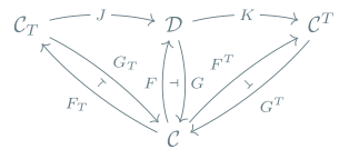We call $K$ the comparison functor. The functor $KJ : \mathcal{C}_T \rightarrow \mathcal{C}^T$ is full and faithful. The Kleisli category is then the initial decomposition of a monad into an adjunction. And likewise, the Eilenberg-Moore category is the terminal decomposition of a monad into an adjunction.